I present here a few mathematical details about vortex flows
A number of mathematical subtleties are linked to the dipole.
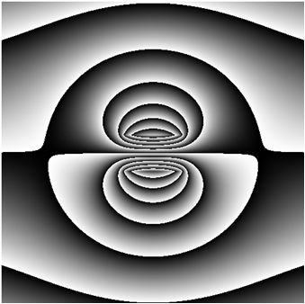
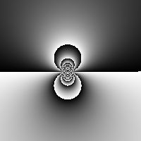
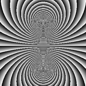
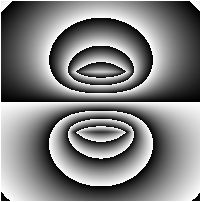
First, one should distinguish the kinetics, and the dynamics. This is to say : the velocities of the flow, and the forces which pull the flow. An incompressible fluid is characterized by the conservation law div(V)=0, which can actually be obtained with different forces. For example, in a tube div(V)=0 implies that the fluid speed is constant. That can be obtained either by pushing at one side, or pulling at the other side.The image to the right shows the scalar values of Y(x,y), coded with a repeated grayscale (values modulo 256). Notice that the values on the upper half and lower half are inverted. This is normal since the vortices revolve in opposite direction, by symmetry.
Classical mathematics/physics of vector fields allows one to define a vector potential A which is perpendicular to the plane of the flow.
A=(0,0,Y(x,y)) such that the third component is a scalar satisfying V=curl((0,0,Y(x,y)).
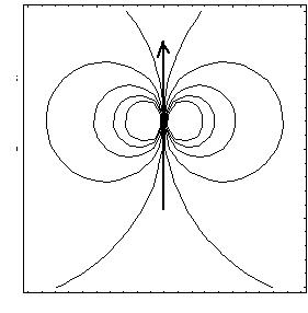
The scalar function Y is called the stream function, and its iso-value curves are the streamlines.
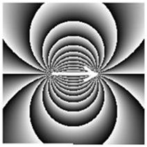
This comes from the fact that the lines of grad(Y) and of curl(Y) are orthogonal. The figure to the right shows a few streamlines of a flow generated by a force located in the center (arrow).
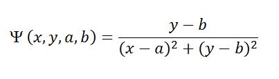
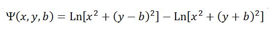
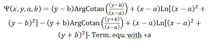
The mathematical formula for the dipole, in (x,y) coordinates, the axis Ox being along the force, and Oy being perpendicular to the force direction.
Note that the speed is infinite in the center. This is a "singularity", which is removed either physically by some other physics in that area (finite size effects, inertia terms, etc.) or mathematically by some "regularization", in terms of distribution functions.
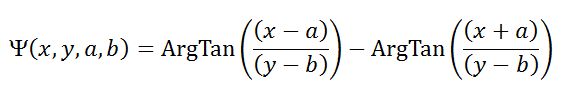
Please note that the result of a uniform pull along a segment, is actually the sum of two vortices exerted at each end, a quite remarkable fact.
In this formula, -b and +b are the location of the center of the vortices along the axis Oy.
Please note that they form some sort of a funnel. By conservation law, the fluid accelerates in the funel. The difference with the single force pulling, is essentially that the funnel is wide (width 2b) therefore the singularity in the nip of the funnel is removed.
However, the flow is still singular in the core of the vortices.
Please note that it is actually the sum of two skewed monopoles located at each end of the line.
The virtue of this function is to elongate the vortices in proportion to the length of the segment
When implementing this into the Stokes equation, one finds a compatibility condition, which is that the speed u(M) for each center M, is the speed V(M), exerted at M, by the OTHER vortices.
Therefore, one generally finds moving vortices. Vortices are not stationary solutions of hydrodynamic equations.
A classical example is the vortex ring (smoke ring).

This I believe, is the explanation of limb bud formation, which has a lenticular shape, and of the navel formation (stagnation point).